Bad Visualization Example: Morning Rush
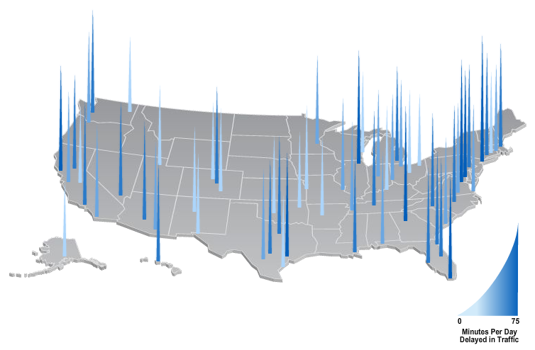
Finding bad visualization wasn’t really a problem as there are plenty of them. I picked this from the Time magzine. The screenshot for the visualization is given below and it tried to show the average commute time for major U.S. cities. One thing not shown in the snapshot is the hover menu that pops-up as soon as you take the mouse over any of the bars. It shows the average delay in numbers.
 Critique:
From Tamara Munzner’s guidelines:
(i) It used color saturation to show quantitative data i.e. average delay time. The interpretation of saturation is shown at the bottom right corner.
(ii) This is an extremely bad use of 3D representation. The given representation suffers from both occlusion and perspective distortion. The average delay values of many of the cities are hidden behind one another, whereas, the height of the bar doesn’t help with any sort of comparison.
From Tufte’s guidelines:
(i) They didn’t mention the source of the data and additionally it is not clear from the context as well.
(ii) Tufte also stress that if visualization is even being published by an organization the name of the individuals who designed it should be mentioned. In context of research paper, I guess it becomes implicit but here it is not.
Overall, this visualization doesn’t provide any information then to act as a graphical look-up (table) for average delay values across major cities. Even if the sole purpose was to offer a nice presentation, I think Time could have done a better job then this.
Good Visualization Example: LiveRAC
This one is from one of the PhD student of Munzner and this work is also related to AT&T vis research group. The link to the paper is here.
Critique:
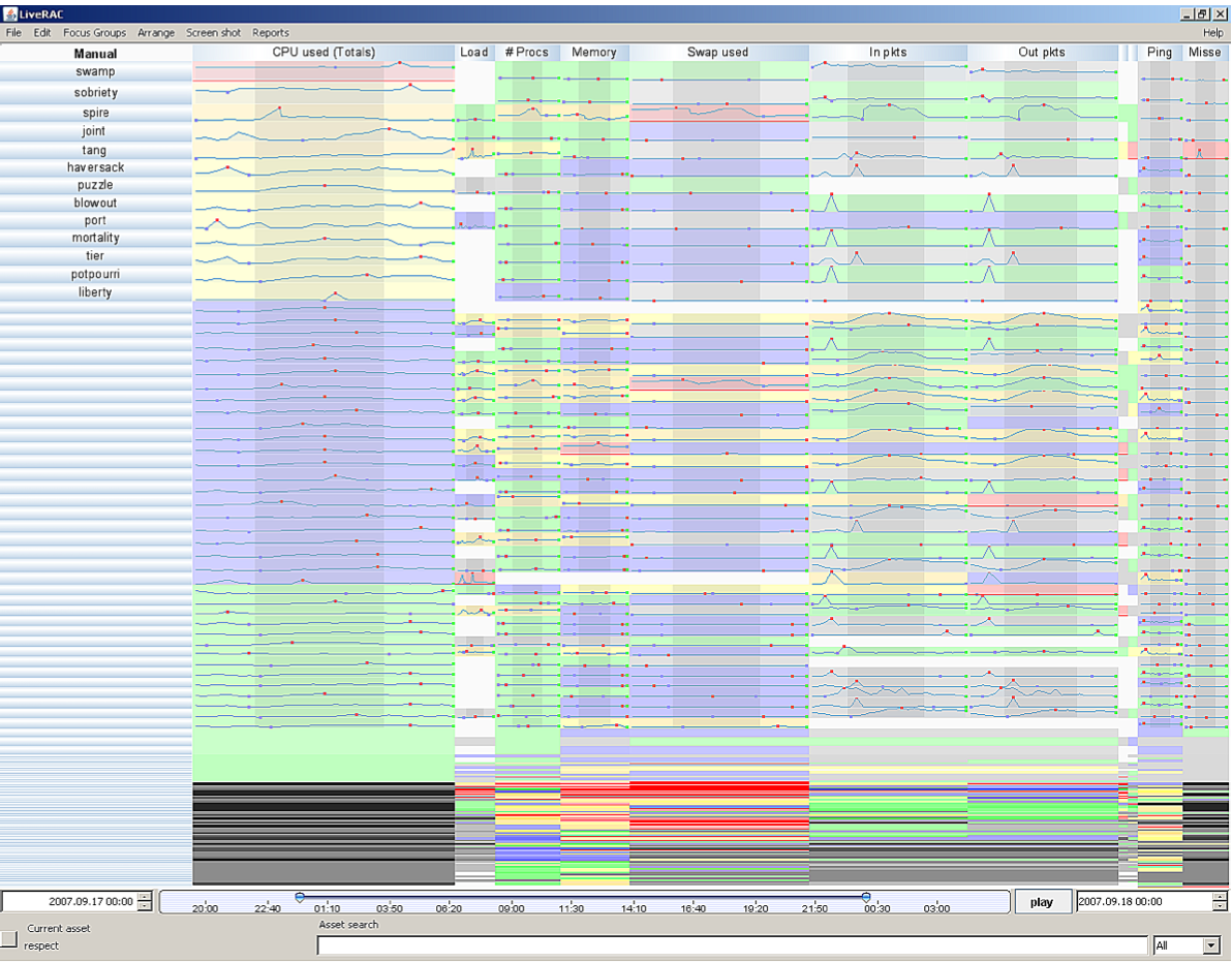
There are generally a large number of system monitoring parameters that are of interest to system administrators. Often these parameters don’t form a pattern or correlation among each other. For example, the large number of input network packets might not necessarily be related to number of processes present in the system or even cluster of systems during a given time period. But, sometime seeing those together and across a cluster might help quickly detect and fix problems. The magnitude of system monitoring information can also pose serious problem So, I think the above visualization does a pretty good job and is an effective use of time series plot.
Each row shows one physical device with columns showing time-series plot for individual parameters. Each column can be sorted and an interval can be highlighted across all columns. One of their design principal was of ‘overview first and then zoom’. Following this each row can be expanded to see the full plots. They have also used color encodings to show the threshold of values in each row. The rows( or devices) that are not fully visible the color value indicates the magnitude of the value for the given parameter ranging from higher (red) to lower(gray) value. This allow us to easily zoom-in to the set of nodes that are showing higher values for a given parameters and then zoom-in further to see the full details (cool!).
{ 1 comment }
I agree with Facial on the bad part of the first plot. It seems to me there are only 3-4 different colors at the first glance. Also, the baseline difference makes it hard to compare the length of each city. Moreover, the goal is to present the average commute time for major U.S. cities, but it does not list the cities names (I cannot distinguish some of them in eastern coast).
For the screenshot of LiveRAC, I think it clearly shows the required information to users. Since the data are time-related, the visualization reflects the variable change against time. As Facial pointed out, each row can be expanded to see the full version, which is another advantage comparing with static plots. I am curious about how large is the dataset, how many rows are there approximately and whether the rows are correlated.