
Tutorial Tableau Walkthrough 2: Life Expectancy
A quick walkthrough of showing how to get started with Tableau. The data set is one we will use in CS765 Fall 2025: Life expectancy data from around the world. I won’t get as far as making “good” visualizations - but it will give you some hints on how to get started with the data set, and with Tableau.
Caveat: I am not a Tableau expert. This is mainly a quick experiment to make sure that it is easy for a Tableau non-expert to work with the data set, and to get to an interesting starting point for actual visualization. This is all with the 2025 version of Tableau Desktop for a Mac, and the data that I am getting from the University of Vienna.
Caveat 2: A lot of this is “what are the easy visualizations to make” not necessarily “what are good visualizations to make.” The goal here was to get an initial sense of a new data set (and some Tableau practice).
Caveat 3: These are quick screen shots (since I often was trying to capture the interface). No effort went in to tuning things to make them look nice. If you are a student in class, you should make sure your visualizations (at least) have titles and captions and legends. Also you probably want to use export (rather than doing a screen capture) and not show the Tableau interface.
Step 1 - Get Some Data Into Tableau
For the class assignment, we’ll work with life expectancy data taken from a class assignment at the University of Vienna.
Here is the data as a CSV file: life-expectancy.csv.
It’s usually a good idea to have a look at the data to have a sense of what to expect. Here, the file is simple: there are just 4 columns.
- Entity
- Code
- Year
- Period life expectancy at birth - Sex: all - Age: 0
Note that the shape of the table is “tall” - each data point is a separate row. We need to look over a lot of rows to see something like “what data is there about the United States” or “what is the data about 1970”. Tall data is convenient in that it can quickly be transformed in to other things.
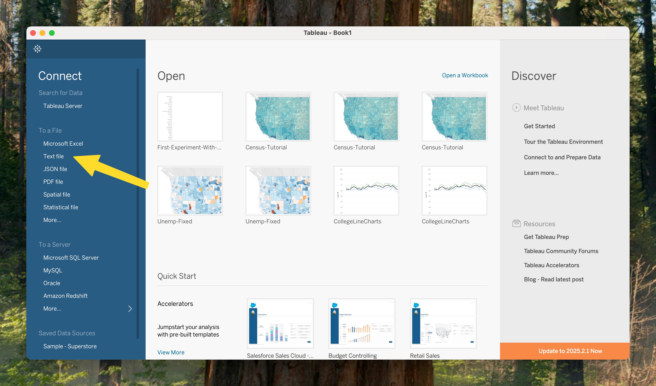
So, I’ll fire up Tableau, and pick “Text File” from the list of connections.
Step 2 - Tell Tableau about the Data
A trick with Tableau is to make sure it knows as much as possible about your data so that it can make good choices without you telling it.
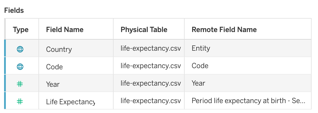
It is pretty good at guessing what is in each column:

But, a few tweaks:
- Telling it that “Entity” and “Code” are countries will help it know to put things on the map (right now, it assumes they are strings). To do this, pick the type (it is text or “Abc”) and change it to “Geographic Role - Country/Region”.
- Turning the year into a date isn’t useful (it will arbitrarily pick a month/dat) - but telling Tableau it is a whole number can help it make better decisions.

- I am changing the “Field Names” to something I like better (Country and Life Expectancy)
Step 3 - Let’s see what’s there!
Now we can make a visualization - my goal is to get a sense of what is in the data set. What countries and years are in the data set?
I’ll click on Sheet 1 (at the bottom) to get a blank worksheet.
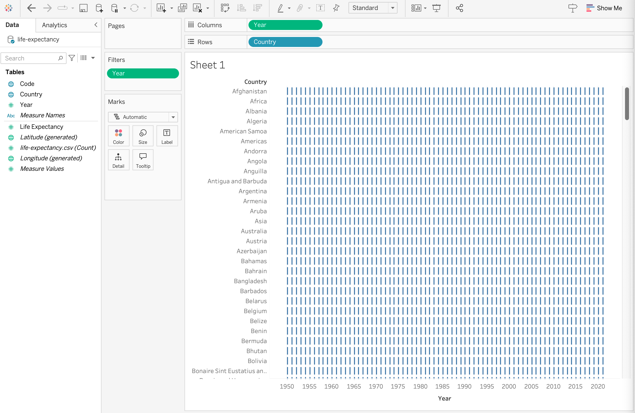
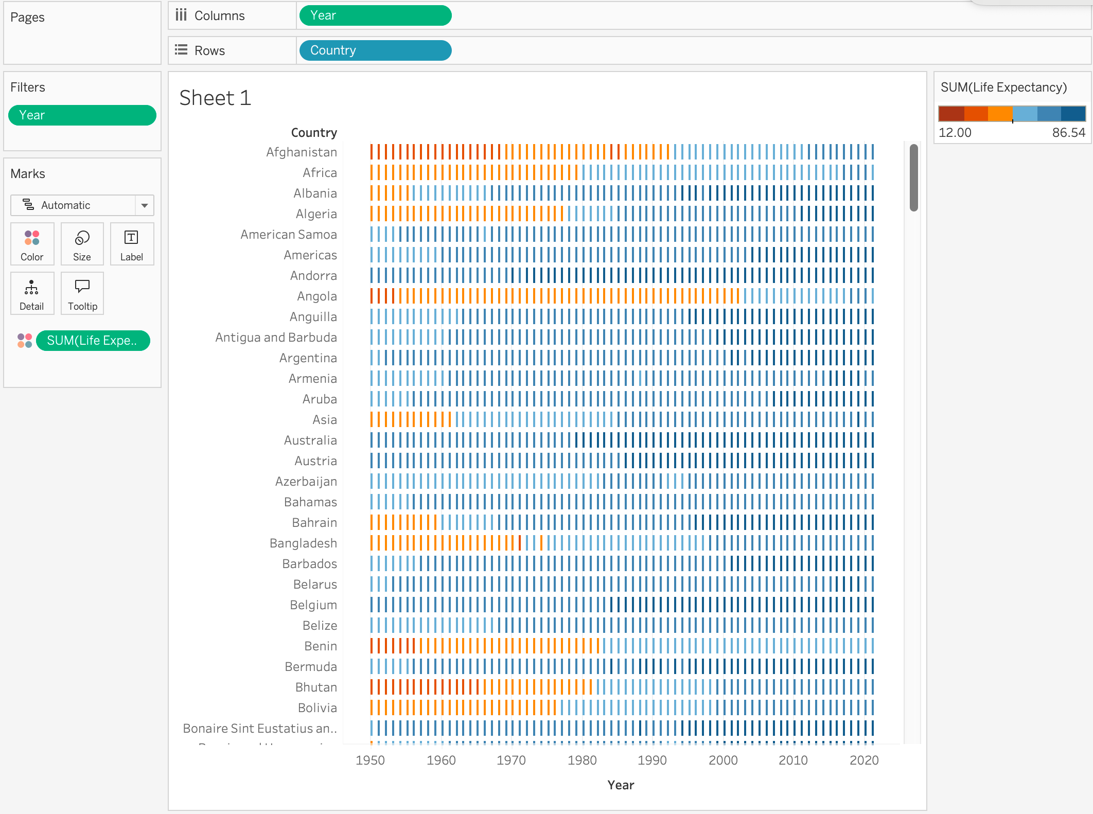
I’ll drop country on the row shelf, and year on the column shelf, and viola! A visualization!

It’s worth pausing for a minute to think about what this is showing us. It’s actually a table (or grid view) that has a mark for which combinations of country and year we have data.
What can you see in this visualization? (take a minute to look at it - even if you’re just reading along).
The first thing I notice is that there is a wide range of years (1550?). If I scroll down, I can see that for the United Kingdom (and only the UK), there is data going back to the 1500s. If I want to compare with other countries, I should probably pick a more narrow range of dates.
At a glance, I can see that for most countries, we have “dense” data (seemingly every year) from around 1950.
So, we’ll focus on 1950 and after… I’ll make a filter by dropping “year” on the filters region, and setting the range to begin in 1950. We get a very different picture, where most countries have data for most years:
Not an amazing visualization - but a useful one. I have a sense of how complete my data is. Now, I want to make a sanity check visualization to see if the data makes sense.
An easy one: I’ll color the marks by life expectancy…
To do this…
- I drop Life Expectancy onto the color symbol (in the marks area). I see something quickly. The scale shows me quite a range (someplace had a 12 year life expectancy?) but it’s hard to see much with the colors. (the subtleties of the blue shadings are hard to see on the small marks).
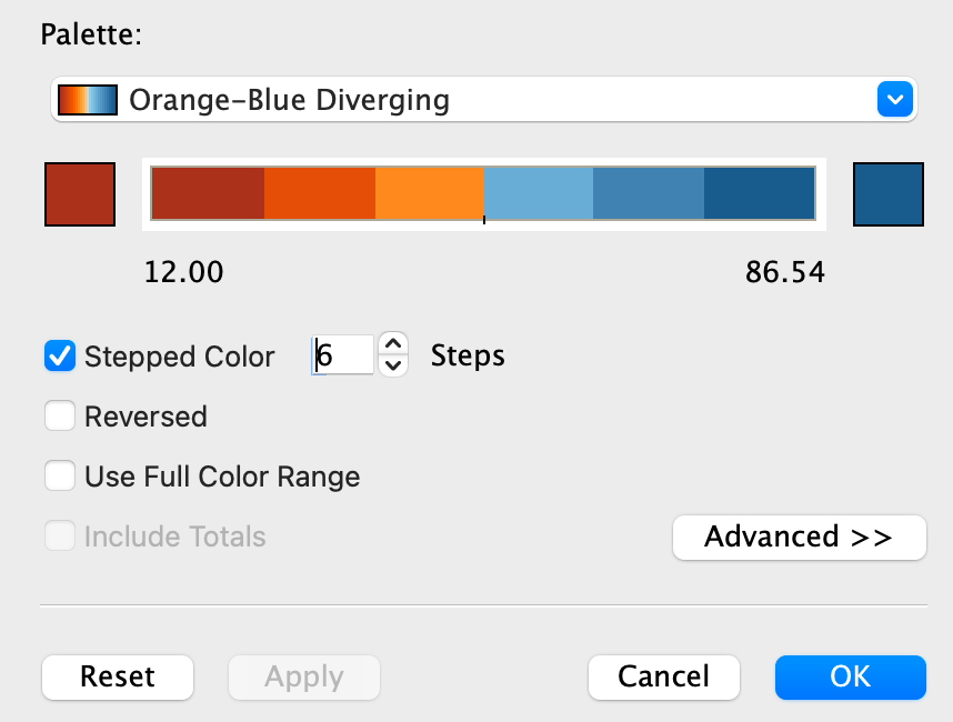
- I change the colors… (double click on the color legend). I am going to pick an orange-blue diverging scale - not that the data is diverging, but it gives me more variety in color (important given the small marks). I am also going to make it 6 steps (so there’s no white in the middle).
I don’t think this visualization is particularly effective for any particular task. But, it was easy to make. And for a quick glance “what’s here”, I think it is useful.
What does this let you see in the data?
An important Tableau detail: notice that the aggregation here is sum, so each mark is summing all data that applies to it. In this chart, each mark is a specific year/country, so there should only be one number. But, (1) it might make more sense to pick the maximum aggregation (so we get just one), or we can pick the count aggregation to make sure that everything has 1 (or zero) data elements. (indeed, it does - phew!)
Step 4 - Some Other Views
Here I am trying to make some of the “standard” ways to look at this data. In part to show how these things are easy to make - and to get a sense of what they are useful for.
4.A: Maps
Let’s try to get a sense of how well the world is covered…
I’ll make a map - showing which countries are in the data set. The easiest way I know to do this is to pick the country field, and then use the “show me” palette to pick map.
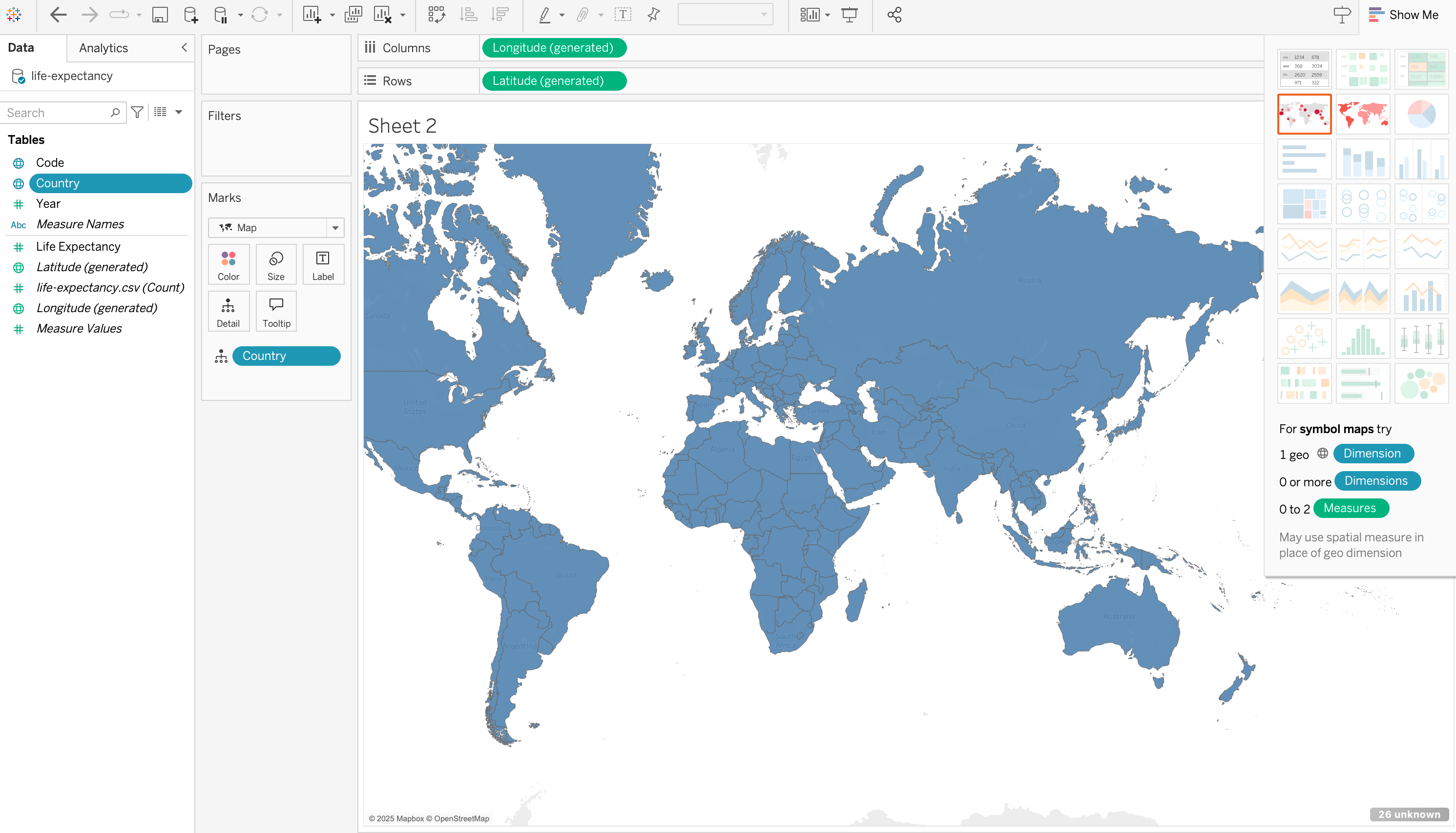
A country is colored blue if there are any data elements for it. Seems like pretty good coverage.
Now, we can drag the “life expectancy” field to color. When we do this, we have a problem (see if you can notice):
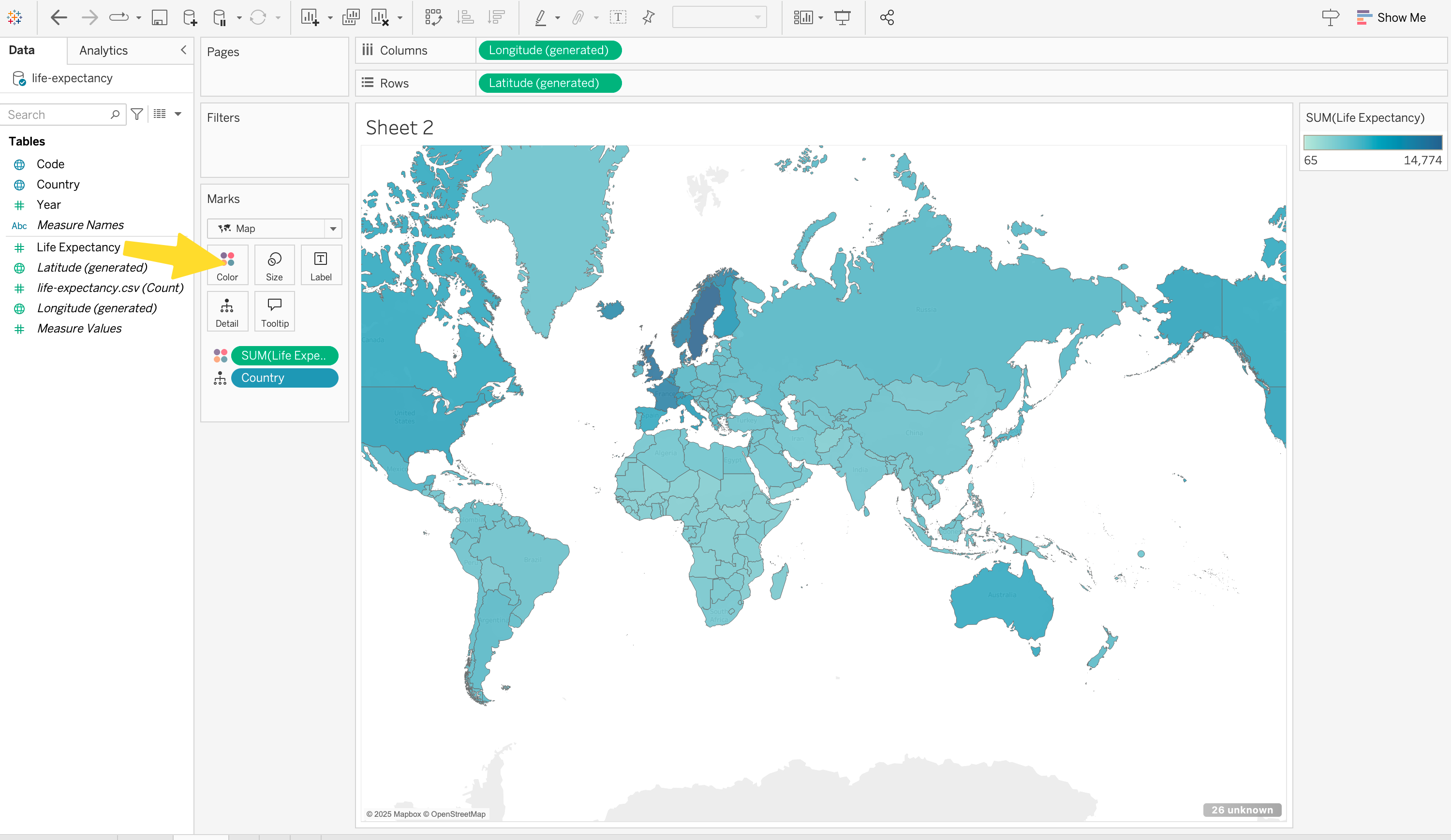
Because the default aggregation is sum, what is being shown is the sum of the life expectance across the years. In most cases, this is similar to the average (because most countries have all 30 years) - but not all countries have 30 years. In fact, we can change sum to count to check this…
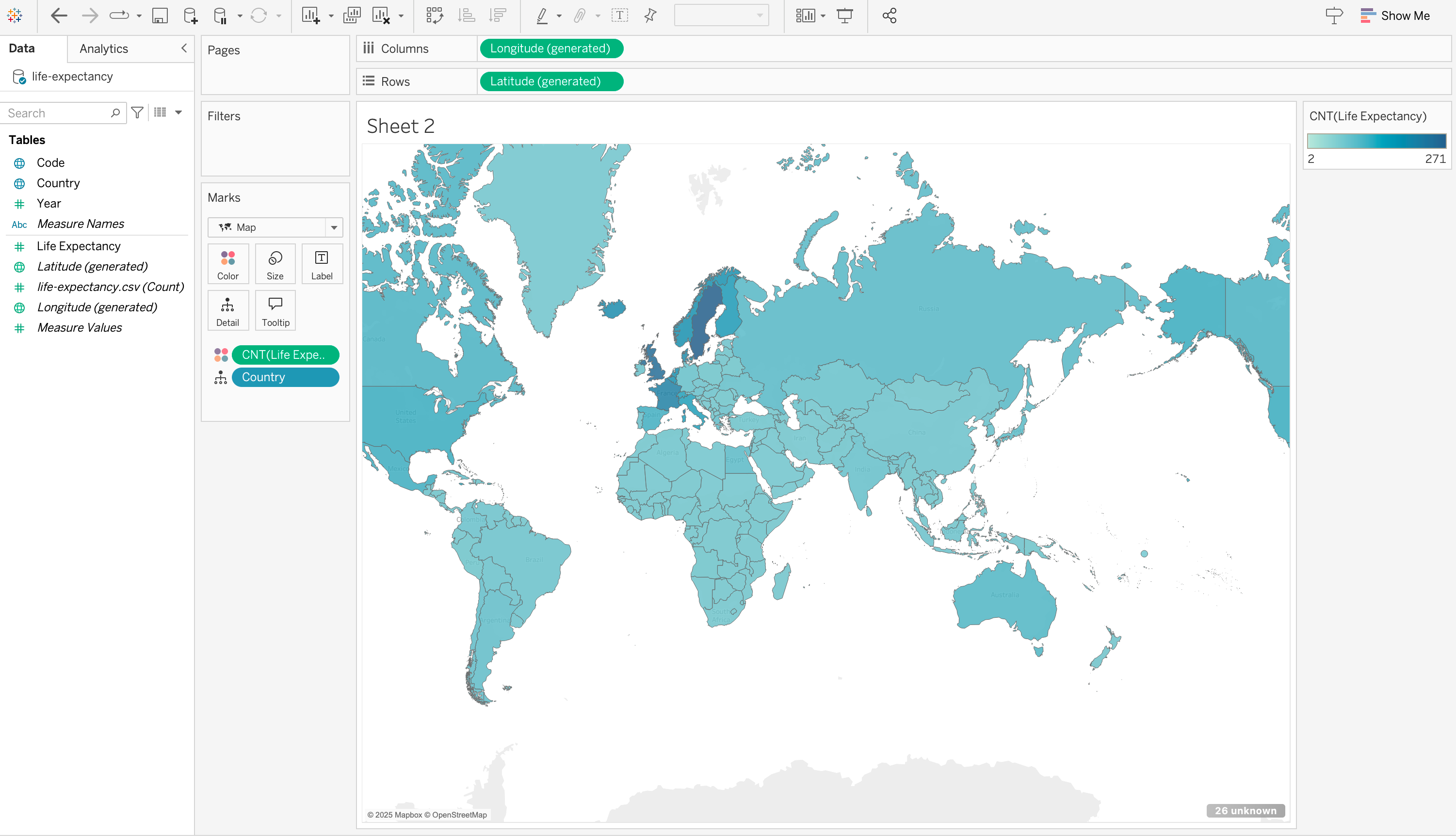
Oh - a reminder that I forgot to put the filter on years (limiting myself to 1950 to the present)…

Putting the filter back is reassuring - all countries seem to have all 72 years.
So, with the filter in place, a sum aggregation makes sense - it’s basically the same as average, except that all the numbers are multiplies by 72. It looks better to pick average (so that the number show up nicely, and it is more obviously sensible). I am more curious about minimum…
Yes, there is a country that in one year had a life expectance of 12 years. Pretty horrible… I wonder if that was just a one off or a persistant problem. I guess we need to look at things over time.
4.B Spaghetti Plot
Spaghetti plot is a perjorative term for a line graph that includes so many lines that they tangle together that it’s hard to see much in any one. That’s not to say they are totally useless - but it goes in the “dump all the data and hope something comes out” categories.
It’s easy to make with this data in Tableau, so I’ll try it…
- Filter Years (I am only doing 1950-2021).
- Drag Life Expectancy to the rows shelf
- Drag Year to the columns shelf
With this, you get a line graph - of the sum of all of the entries for the year. Just as the map summed over years (per country), this is summed over the countries (in a year). We could pick a better aggregation, but instead, I am going to dis-aggregate.
- Drag country to color. Note that it will tell us it’s a bad idea - which we should know! We have 261 “countries” - we can’t give each a unique color (in a meaningful way). But we aren’t necessarily trying to make a meaningful chart that shows everything. Just (1) to show we can do it, and (2) get some sense of what’s going on.
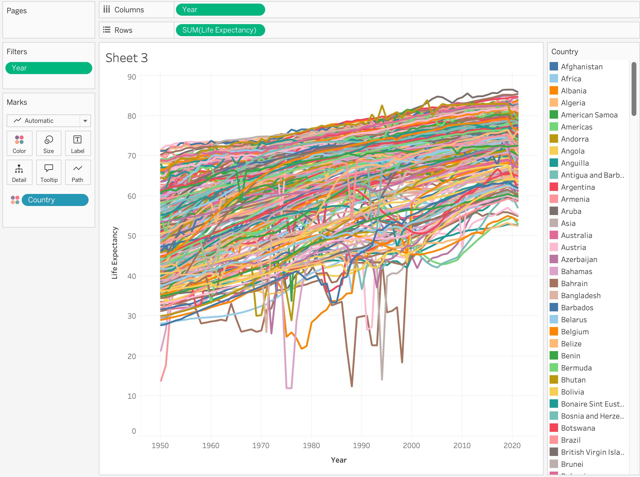
Take a minute to look at this. It’s easy to see what’s wrong. But think about what is right. What can we learn from this (admittedly problematic) visualization that can help us decide where to look farther.
One thing with a “bad” visualization, is that we can use Tableau’s interactivity to help see through the mess. For example, I can click on one of the outliers to figure out what it is…
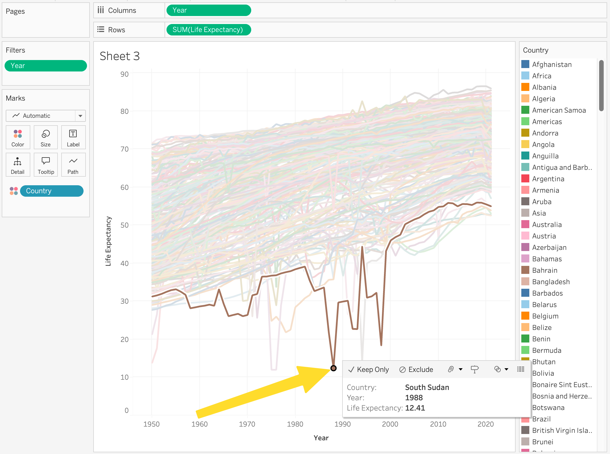
Here I’ve clicked on the point at the bottom - which highlights the line it is part of. The tooltip gives me information about the specific point.
From here, I could try to improve things (for example, by focusing on particular countries). But I’ve already gotten some basic ideas of what is in the data set.
Not So Easy…
So far, I made visualizations that were convenient with the data in the form of the data (and my limited Tableau skills).
The “tall” form of the data makes some things tricky. For example, if I want to look at the differences between two years (which countries have the biggest gains between 2000 and 2018?), each “point” (for a country) requires two data elements (rows). If we had “wide” data (for example, a row per country, a column per year) - we could easily derive another column that is “delta 00 to 18”. (of course, if we had wide data, it would be harder for questions that were year centric).
My Tableau skills don’t give me an easy way to do the “compute something over several rows”. To be honest, my fallback is to write a script (probably python) and compute a different data table in a convenient “wide” format. There are ways to do this in Tableau, it’s just beyond my skillset at the moment.
So, with a little help from a friendly chatbot (Gemini - see AI disclaimer below), I was able to make a chart of “which countries have the biggest change” by…
- Defining a new calculated field “1950” that selects rows for year 1950.
if [Year] = 1950 THEN [Life Expectancy] END - Defining a new calculated field “2021” (similar)
- Defining a new calculated field “Change” (and this is a tricky part) as
SUM([2021]) - SUM([1950]). Note that this aggregates over all rows. I could have used Max instead - Using this new field in a chart (dragging it to the row, with country as a column)
- Sorting the chart’s X as by the change

The new “change” variable can make a nice map as well…