Dataset: This use case considers a corpus of 59,989 documents from a historical literary collection and the data counts the 500 most common English words in each document.
Classifiers: The classifiers for this task are decision tree classifiers using a variety of univariate feature selection strategies, each selecting 10 words to count for features. The feature selection methods were: most relevant by a CHI-squared univariate feature selector (C), most common features (N), randomly chosen features (R), and, as a baseline, the features deemed worst (out of the 500 candidate words) by the CHI-squared test (W).
Walkthrough:
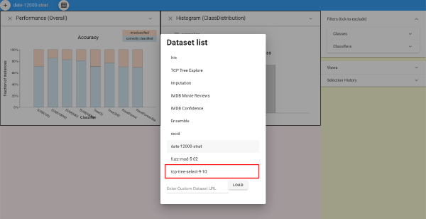
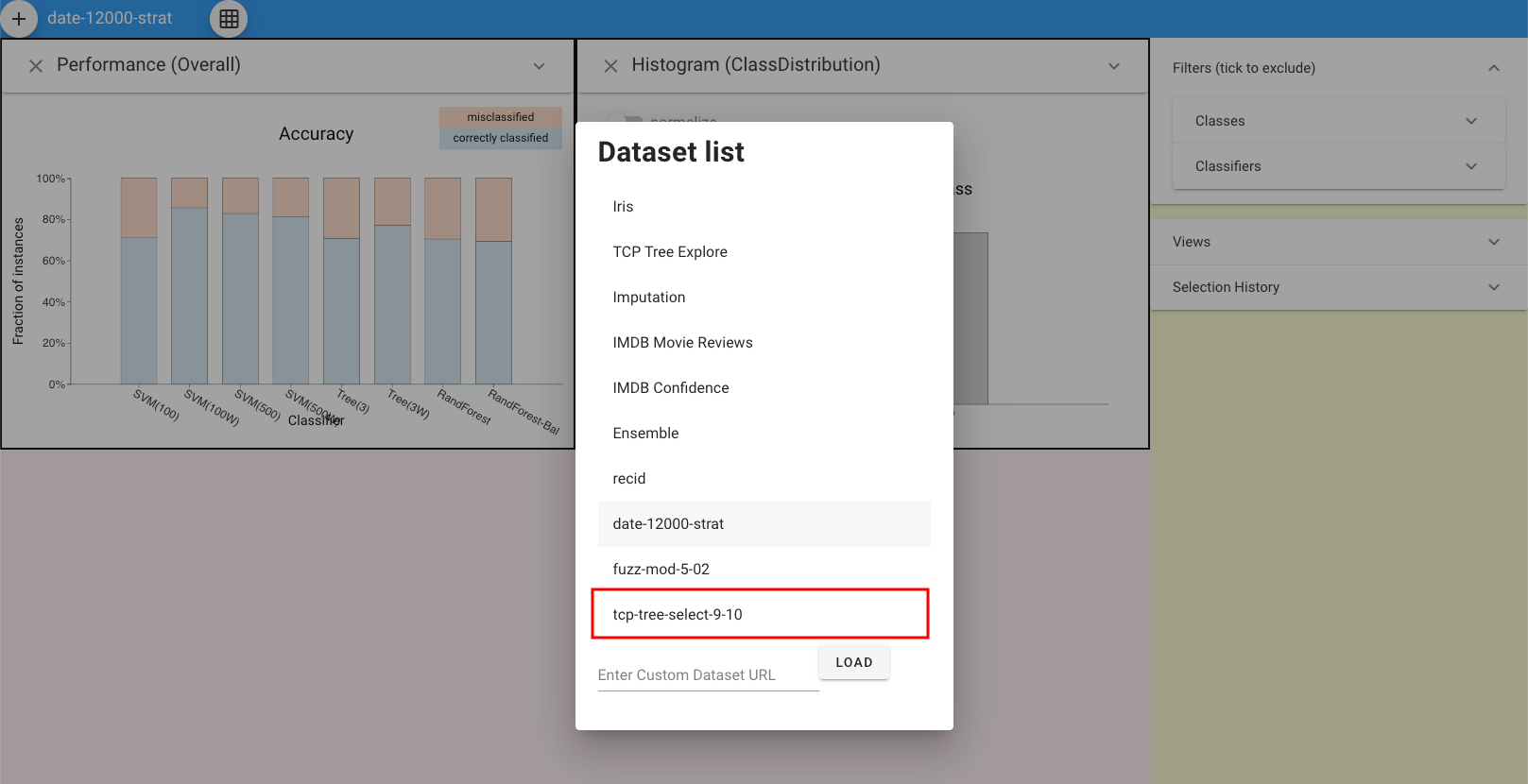
First, click the button on the top left and load the dataset.
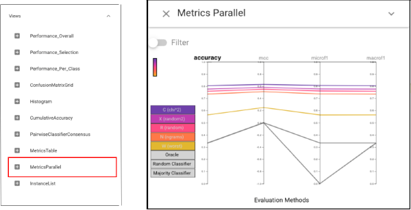
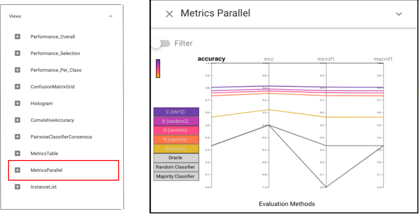
In order to have an overview of performances of each classifier, we can first choose the Metrics Parallel view.The Parallel Metrics view shows a consistent ordering of the classifiers across all metrics: C is slightly better than R and N, which are much better than W.
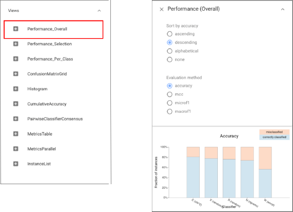
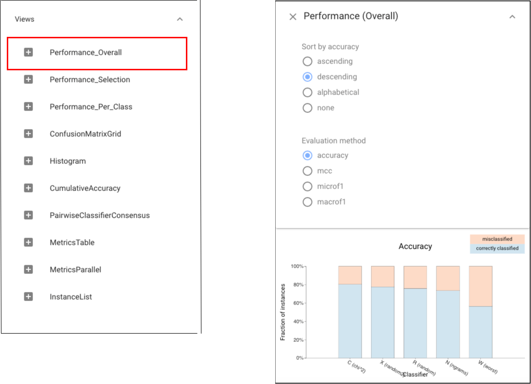
Then we can apply Classifier Performance here to see the accuracy details of each classifier:
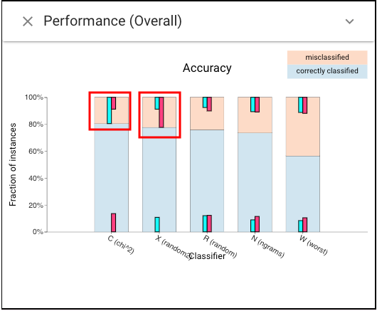
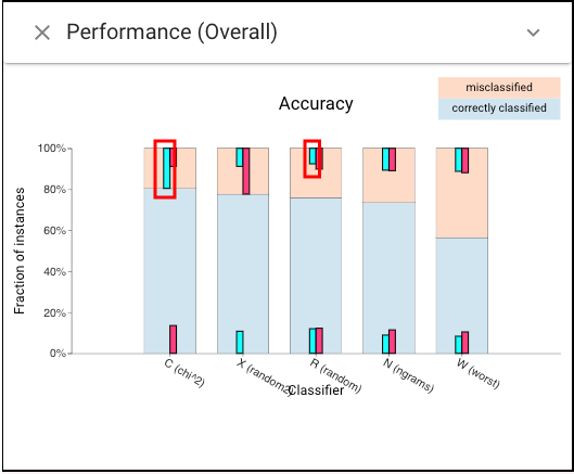
Next, let’t make some selections. We can select the mistakes made by the top classifiers (cyan for C’s mistakes, and magenta for X’s mistakes):
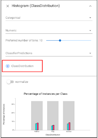
In order to see the error’s distribution on different classes, we can open the Histogram view and focus on the class distribution:we find that the errors are relatively evenly distributed among the classes and this is surprising given the skewed training distribution.
We also see in the Classifier Performance view that different classifiers make different errors (e.g., only half of C’s errors are made by N):
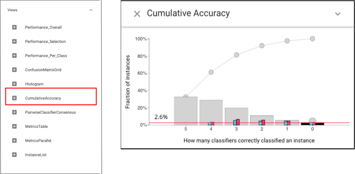
To select challenging instances, or to see if a selected set contains easy items, we can use Cumulative Accuracy view:Overall, the Cumulative Accuracy view shows that there are very few instances that all classifiers were wrong on (2.6%).
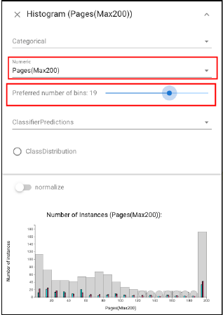
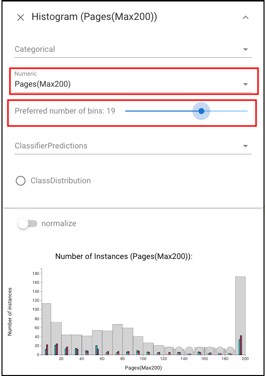
Let’s back to Histogram view and focus on the error distribution on specific features. Open a Histogram view of document lengths and drag the slider to change the number o bins:and we can see that performance is relatively consistent over the range of document lengths.