Data Examination #
Dataset: This use case considers a corpus of 59,989 documents from a historical literary collection: Text Creation Partnership (TCP) transcriptions of the Early English Books Online (EEBO). The data counts the 500 most common English words in each document. For the experiment, we took a random sample of 2500 documents, and held out 30% using stratified sampling.
Classifiers: We construct classifiers that determine whether a document is written after 1642 based on the 500 most common words in the corpus. We constructed random forest (RF) and logistic regression classifiers (LR), with and without applying corrections for class skew.
Walkthrough: While ground truth is known, effective classifiers can help understand how word usage changed at this critical date that marks the beginning of the English Civil War. The collection is skewed (only 25% of the documents were written before 1642). Therefore, we prefer MCC as a correctness metric.
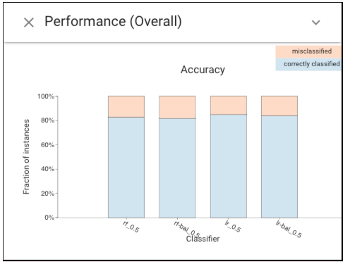
Based on Performance Overall view, the random forest classifiers achieve worse performance with the default (.5) threshold on the test set.
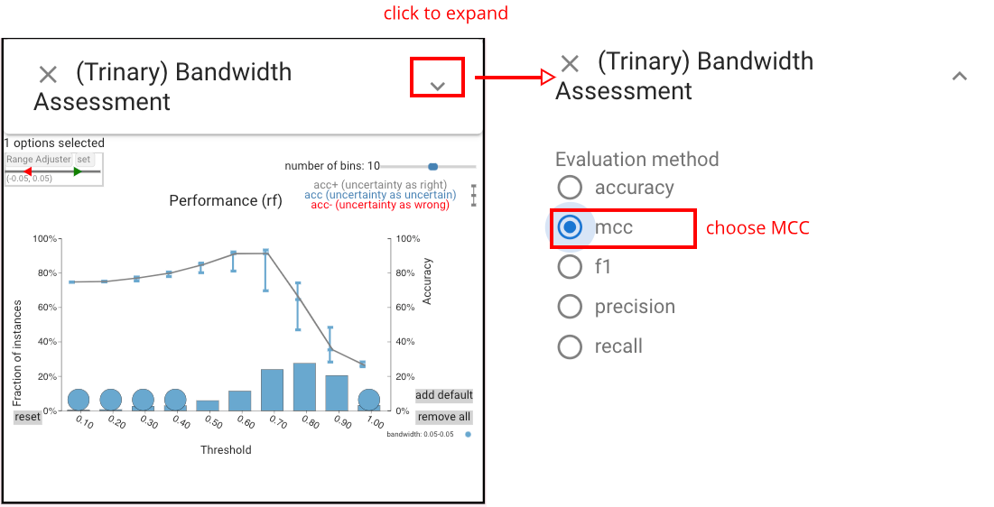
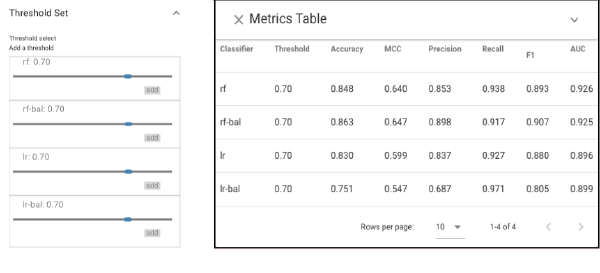
Since we prefer to using MCC as correctness metric, we need to set classifiers' thresholds based on their MCC values. Using the Bandwidth Assessment view we can choose the threshold that optimizes MCC for each classifier.
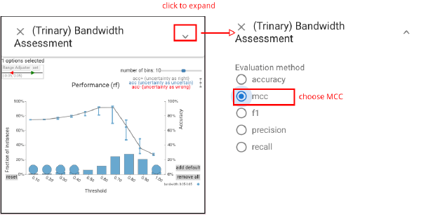
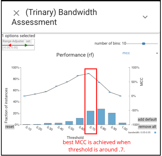
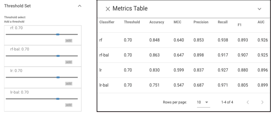
Based on our findings in Bandwidth Assessment view, we set all classifiers' thresholds as .7 (the following graph shows the how MCC changes with threhsold of classifier rf).
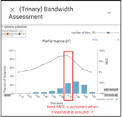
Now, we can tell that after choosing the threshold that achieves the highest MCC for each classifier, the RF classifiers have the best performance across metrics.
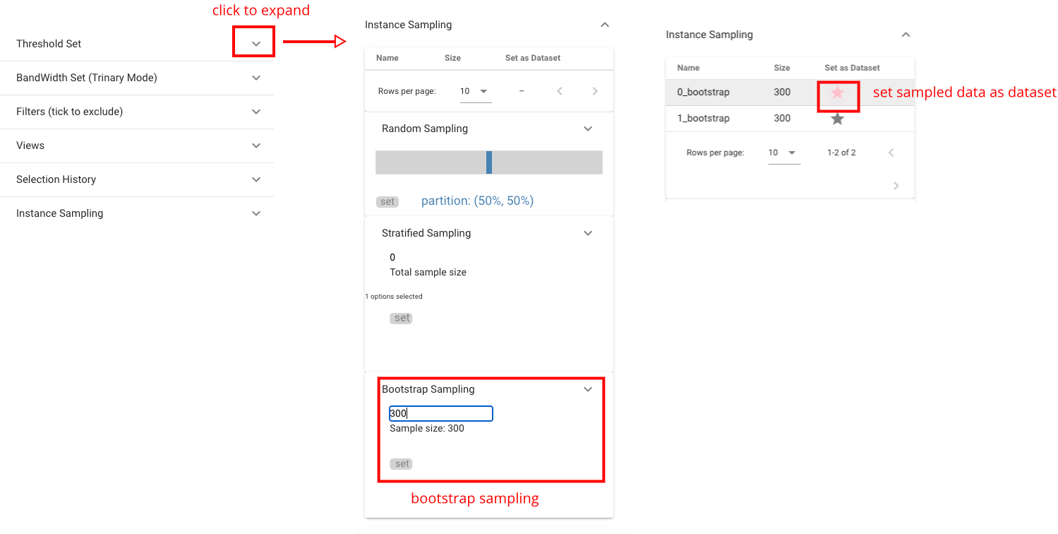
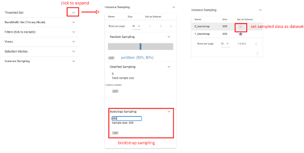
However, this optimized performance may be specific to the test set. To provide a check against overfitting, we use CBoxer’s bootstrap sampling feature to create 10 new testing sets from the original (the following graph shows how to use Instance Sampling panel to create samples) and see that the results do not change. While the precise values of threshold and metrics may change, in all cases, RF beats LR.
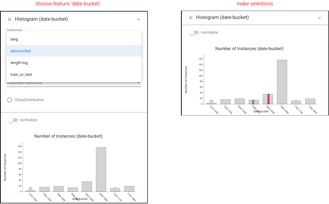
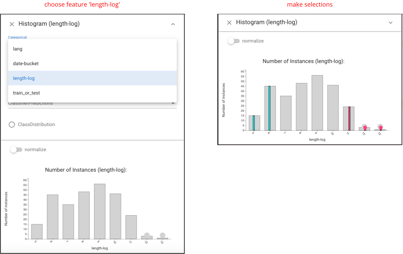
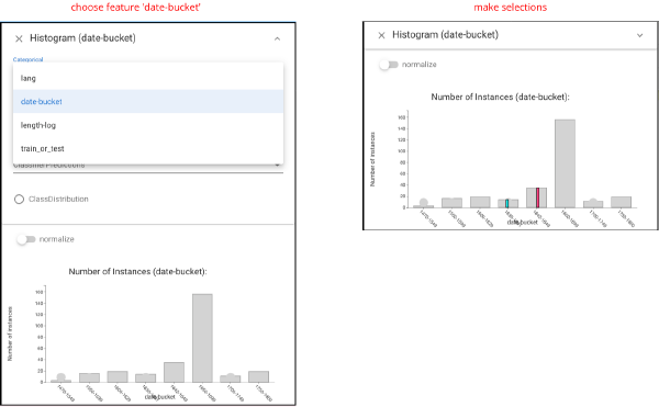
A question is whether performance near the boundary is different than documents written farther from the critical date. We can select the time periods before and after the critical date by using Histogram view
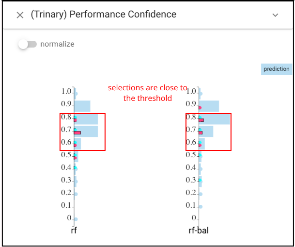
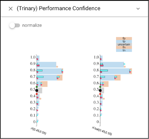
Then under the ‘original distribution’ mode of the Performance Confidence view, we can see that the scores are generally closer to the threshold. Both before and after the boundary seem to be problematic which suggests that language was in flux before the English civil war.

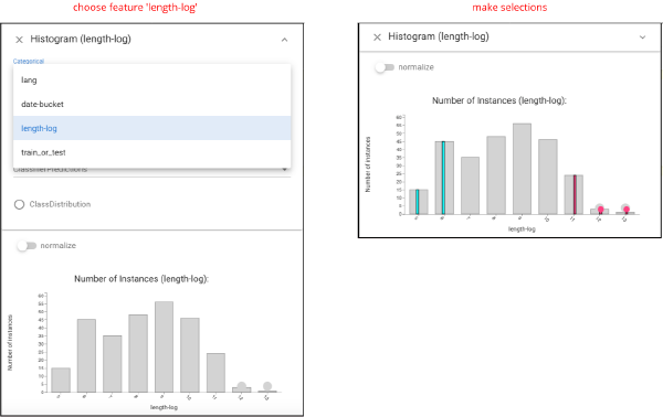
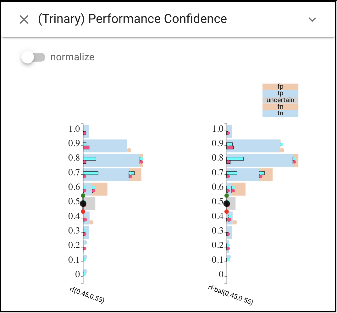
Another question is whether the length of documents has any connection to the certainty of a prediction. Using a Histogram view, Let’s select the shortest and longest documents. Then we can view the distribution over Performance Confidence view.
We can see that long documents are disproportionately given confident scores, while the shortest documents (less than 150 words) score in the center (less confident predictions).